There’s an equation that comes up a lot in optimization literature contexts. It’s part of the Karush–Kuhn-Tucker (KKT) conditions for first-order optimality for systems with multiple equality and inequality constraints. It’s used in dynamics. I’m talking about the Lagrangian. Just seeing where it pops up as been a useful touchstone in further reading for me.
The first exposure most of us had to the Lagrangian is through Lagrange Multipliers. Before that, a very brief refresher on the derivative and function extrema:
The extrema of a continuous, differentiable function \(f(x)\) along the interval \([a, b]\) occurs at one of the critical points, which are the endpoints and any point between \(a, b\) where \(f'(x)=0\).
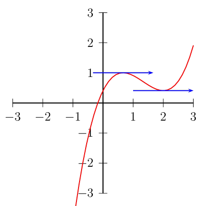
Here we see a graph of \(f(x) = \frac{1}{2}x^3 - 2x^2 + 2x + 0.41\) between –3 and 3. The points at which the tangent of \(f\) is 0 have the blue lines. If we want to find either the maximum or minimum value of \(f\) over 0 to 3, it suffices to test the value of \(f\) at 0, those two points (\(x=\frac{2}{3}, 2\)), and 3. This follows from the fact that the tangent before an extrema and the tangent after must have different signs, and since \(f\) is continuous the point where the tangent switches signs (i.e., is 0) is an extrema.
Similarly you can distinguish whether an extrema is a minimum or maximum by testing the second derivative: if \(f''\) is negative, then the tangent was itself decreasing and on its way to a maximum.
The Lagrange multipler first shows up in multivariable calculus in this context: Given a function f(\textbf{x}) and a constraint g(\textbf{x}), how do we find the maximum value of f such that \(g(\textbf{x}) = 0\)? To find the answer we first to understand the gradient of \(f\).
The gradient helps generalize the concept of the tangent to arbitrary dimensions. Instead of a scalar that defines the tangent line at each point, the gradient is a vector that points in the direction of greatest change for a function. It’s normal to any level curve and so defines the tangent plane in which any tangent line for any level curve must lie. Given \(f(x,y,z)\) the gradient ∇f is defined as \(\begin{bmatrix} \frac{f}{x} & \frac{f}{y} & \frac{f}{z} \end{bmatrix}\).
Here’s an image of the gradient at a point on a sphere:
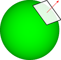
The red arrow illustrates the ∇f at a point \(p\). A level surface, remember, is the set of points where a function takes the same value. A sphere, for example, is described by the level surface \(x^2+y^2+z^2=k\). In arbitrary dimensions the level surface is called a level curve.
Back to the original question: Given \(f(\textbf{x})\) and \(g(\textbf{x})=0\) it turns out, if \(f\) and \(g\) intersect at all, \(f\) takes a maximum at a point \(p\) where the gradients for \(f\) and \(g\) are parallel.
Imagine any curve on the sphere that intersects \(p\). At \(p\), the gradient for all curves will be normal to the surface. Another way of putting it is that the tangent of that curve at \(p\) will have to lie in the plane whose basis vectors are orthogonal to (in the null space of) ∇f.
\[\nabla f = \lambda\nabla g\]
To see this, consider \(f(\textbf{x})\) and \(g(\textbf{x})\) such that \(g(\textbf{x})=0\) intersects \(f\). The resulting intersection is a level curve \(g(\textbf{x})=0\), and so ∇g will be normal along its path. For a point \(p_0\) to be the maximum value of \(f\) on this path, then any move along \(f\) away from \(p_0\) must decrease the value of f. Since this is true no matter what curve we picked to go through this path, then all tangents at that point lie in a plane and equivalently, ∇f at \(p_0\) is normal to the curve.
As ∇g and ∇f are normal to the curve at \(p_0\), their respective tangent planes represent the same space. If \(p_0\) exists, \(∇g=\lambda∇f\).
An alternative way of thinking about it follows from calculus. Consider the path through \(f\) such that \(g(\textbf{x})=0\). If we parameterize \(g(\textbf{x})\) with \(x=h(t), y=j(t), z=k(t)\) then this path is \(f(h(t), j(t), k(t))\). The derivative with respect to t is then
\[\frac{df}{dt} = \frac{\partial f}{\partial x} \frac{dh}{dt} + \frac{\partial f}{\partial y} \frac{dj}{dt} + \frac{\partial f}{\partial z} \frac{dk}{dt} = \nabla f \cdot v\]
where \(v\) is the velocity vector.
The maximum along this path occurs when the derivative \(\frac{df}{dt}=0\), or \(\nabla f \cdot v = 0\), that is, when the gradient is orthogonal to the tangent of \(g(\textbf{x})=0\).
The \(\lambda\) in the relationship \(\nabla f = \lambda\nabla g\) is called the Lagrange Multiplier. We know that the gradients, if a extrema point exists where \(f\) and \(g\) intersect, must occur when \(\nabla f\) and \(\nabla g\) are parallel. But their exact proportions are unknown. Indeed, their gradients may even be pointing in opposite (but parallel) directions.
This provides us with a equation for each dimension of x. We need one more equation to account for the additional unknown, λ. In this case we’ll can use the constraint as our last equation, giving us a balanced system which we can solve using the usual methods.
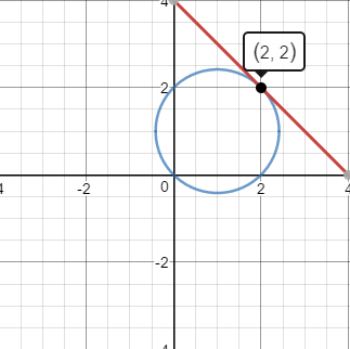
Here’s an image that illustrates the relationship in two dimensions. Consider the circle centered at \((1,1)\) bounded by the line \(x + y = 4\). How big can we make the radius of the circle and have it all on one side of the line? (Equivalently, given a circle that just touches a line, at what point do they intersect?)
To setup the problem, given
\[\begin{align} f(\textbf{x}) &= (x-1)^2 + (y-1)^2 \\ g(\textbf{x}) &= x + y - 4 \end{align}\]
…we’re looking to maximize \(f(\textbf{x})\) such that \(g(\textbf{x})=0\). We’ll do so by finding the spot where f and g have parallel tangents proportional to some \(\lambda\), the Langrange Multiplier. More concisely we express this as \(\nabla f = \lambda\nabla g\).
After applying the gradient via \(\nabla f = \lambda\nabla g\), we have
\[\begin{align} 2 x - 2 &= \lambda \\ 2 y - 2 &= \lambda \end{align}\]
…leaving two equations and three unknowns. We can use g to provide the necessary third equation:
\[x + y = 4\]
This system can easily be solved via substitution, giving us \(\lambda = 2\) and \(x=y=2\). This gives a maximum radius of \(\sqrt{2}\) (Why not \(2\)? Because we characterized f as \(x^2+y^2\), so we were actually solving for \(radius^2\)).
This presentation of the Lagrange multiplier is actually an application of what’s called the Lagrangian function. We can use the Lagrangian to reexpress the problem using one equation:
\[\mathscr{L}(\textbf{x}, \lambda) = f(\textbf{x}) - \lambda g(\textbf{x})\]
To which we apply the gradient, giving
\[\nabla\mathscr{L}(\textbf{x}, \lambda) = \begin{bmatrix} \frac{\partial f}{\partial x} - \lambda \frac{\partial g}{\partial x} & \frac{\partial f}{\partial y} - \lambda \frac{\partial g}{\partial y} & -g \end{bmatrix} = 0\]
… giving us the requisite number of equations to unknowns.
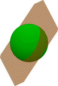
Problem setup isn’t mechanical, it requires some thought. Consider the question of the intersection of the sphere \(x^2+y^2+z^2=2\) and plane \(z = x+y\) in 3d.
A little substitution gives us a set of points along the ellipse of intersection.
\(x^2+y^2+(x-y)^2=2 \implies x^2+y^2+x^2-2xy+y^2=2 \implies x^2-xy+y^2=1\)
Let’s attempt to solve using the Lagrange Multiplier method with \(f=x^2+y^2+z^2-2\) and \(g=x+y-z\). Differentiating gives us
\[\begin{align} \nabla f &= \begin{bmatrix} 2x & 2y & 2z \end{bmatrix} \\ \nabla g &= \lambda \begin{bmatrix} 1 & 1 & -1 \end{bmatrix} \end{align}\]
with a system of three equations with four unknowns.
\[\begin{align} 2x &= \lambda \\ 2y &= \lambda \\ 2z &= \lambda \end{align}\]
See what happens if we use the constraint function as the last equation?
\[\begin{align} x+y-z &= 0 \\ \frac{\lambda}{2} + \frac{\lambda}{2} - \frac{\lambda}{2} &= 0 \end{align}\]
…giving us \(\lambda\) of 0! The problem here was the selection of the last equation: the first three equations tell us that if a maximum \(p=\begin{bmatrix} x &y &z\end{bmatrix}\) exists, \(x=y=z=\frac{\lambda}{2}\) that point. The last equation enforces that that point also lies in the plane. As a result, we solve for a value of x,y,z that lies in the plane with all points equal - that is, 0.
Substituting instead the sphere equation give us:
\[\begin{align} x^2+y^2+z^2 &= 2 \\ (\frac{\lambda}{2})^2 + (\frac{\lambda}{2})^2 + (\frac{-\lambda}{2})^2 &= 2 \\ \frac{3 \lambda^2}{4} &= 2 \\ \lambda^2 &= \frac{8}{3} \\ \lambda &= \pm \sqrt{\frac{8}{3}} \end{align}\]
Giving values of \(\pm \sqrt{\frac{2}{3}}\) for x, y, and z, a solution to the original problem.
It should be clear how to extend the method to multiple dimensions, but what about multiple constraint functions? Consider \(f(\textbf{x})\) subject to \(g(\textbf{x})\), \(h(\textbf{x})\). Unless \(\nabla g\), \(\nabla h\) are parallel, we can solving this problem with multiple constraints using Lagrangian multipliers. Expressed as a Lagrangian:
\[\mathscr{L}(\textbf{x}, \lambda, \mu) = f(\textbf{x}) - \lambda g(\textbf{x}) - \mu h(\textbf{x})\]
Taking the partial derivative of \(\mathscr{L}\) (and assuming \(\textbf{x} = (x, y)\)) gives us four equations:
\[\begin{align} {\frac{\partial\mathscr{L}}{\partial x}} &= \frac{\partial f(\textbf{x})}{\partial x} - \lambda \frac{\partial g(\textbf{x})}{\partial x} - \mu \frac{\partial h(\textbf{x})}{\partial x} \\ {\frac{\partial\mathscr{L}}{\partial y}} &= \frac{\partial f(\textbf{x})}{\partial y} - \lambda \frac{\partial g(\textbf{x})}{\partial y} - \mu \frac{\partial h(\textbf{x})}{\partial y} \\ {\frac{\partial\mathscr{L}}{\partial \lambda}} &= -g(\textbf{x}) \\ {\frac{\partial\mathscr{L}}{\partial \mu}} &= -h(\textbf{x}) \end{align}\]
For example, what are the closest points between the circle \(x^2+y^2=1\) centered around \(2, 2\) and the ellipse \(\frac{2}{3}s^2 + \frac{2}{5}st + \frac{2}{3}t^2 + \frac{3}{4}s+\frac{1}{2}t=2\)? (s and t here correspond to the Cartesian x and y, we picked different letters to distinguish them from the point on the circle).
Since we’re trying to find the closest point, the function we’re looking to optimize will be the distance function. Since we’re looking for the minimum we can just flip the sign.
\[f(x,y,s,t) = -((x-s)^2 + (y-t)^2)\]
Since we are comparing points on the boundaries of our shapes, our constraint functions are simply the level curves of the implicit form (set equal to 0).
\[\begin{align} g(x,y,s,t) &= (x-2)^2+(y-2)^2-1 \\ h(x,y,s,t) &= \frac{2}{3}s^2 + \frac{2}{5}st + \frac{2}{3}t^2 + \frac{3}{4}s+\frac{1}{2}t-2 \end{align}\]
Giving us \[\begin{align} \mathscr{L}(\textbf{x}, \lambda, \mu) &= -((x-s)^2 + (y-t)^2) - \lambda ((x-2)^2+(y-2)^2-1) - \mu (\frac{2}{3}s^2 + \frac{2}{5}st + \frac{2}{3}t^2 + \frac{3}{4}s+\frac{1}{2}t-2) \\ {\frac{\partial\mathscr{L}}{\partial x}} &= (s-x) - \lambda (x-1) \\ {\frac{\partial\mathscr{L}}{\partial y}} &= (t-y) - \lambda (y-1) \\ {\frac{\partial\mathscr{L}}{\partial s}} &= 2(x-s) - \mu \frac{4}{3}s + \frac{2}{5}t + \frac{3}{4} \\ {\frac{\partial\mathscr{L}}{\partial t}} &= 2(y-t) - \mu \frac{4}{3}s + \frac{2}{5}t + \frac{1}{2} \\ {\frac{\partial\mathscr{L}}{\partial \lambda}} &= -((x-2)^2+(y-b)^2-1) \\ {\frac{\partial\mathscr{L}}{\partial \mu}} &= -(\frac{2}{3}s^2 + \frac{2}{5}st + \frac{2}{3}t^2 + \frac{3}{4}s+\frac{1}{2}t-2) \end{align}\]
Setting the left hand side to 0 gives us a non-linear system of equations. No fun to solve by hand but easy enough to plug into a numeric solver.
\[\begin{align} x ~&= 1.265081 \\ y ~&= 1.321845 \\ s ~&= 0.725846 \\ t ~&= 0.824260 \end{align}\]
My go-to calculus reference.
In case you need convincing that the gradient is, indeed, perpendicular to a level curve here you go.
-- Joe Valenzuela (Senior Engine Programmer)